# pylint: disable=missing-module-docstring,invalid-name

from collections.abc import Callable
from typing import Optional

from treat_sim.model import Scenario, single_run
from sim_tools.output_analysis import (
    ReplicationsAlgorithm,
    ReplicationsAlgorithmModelAdapter,
    ReplicationTabulizer,
    plotly_confidence_interval_method,
)Automating the selection of the number of replications
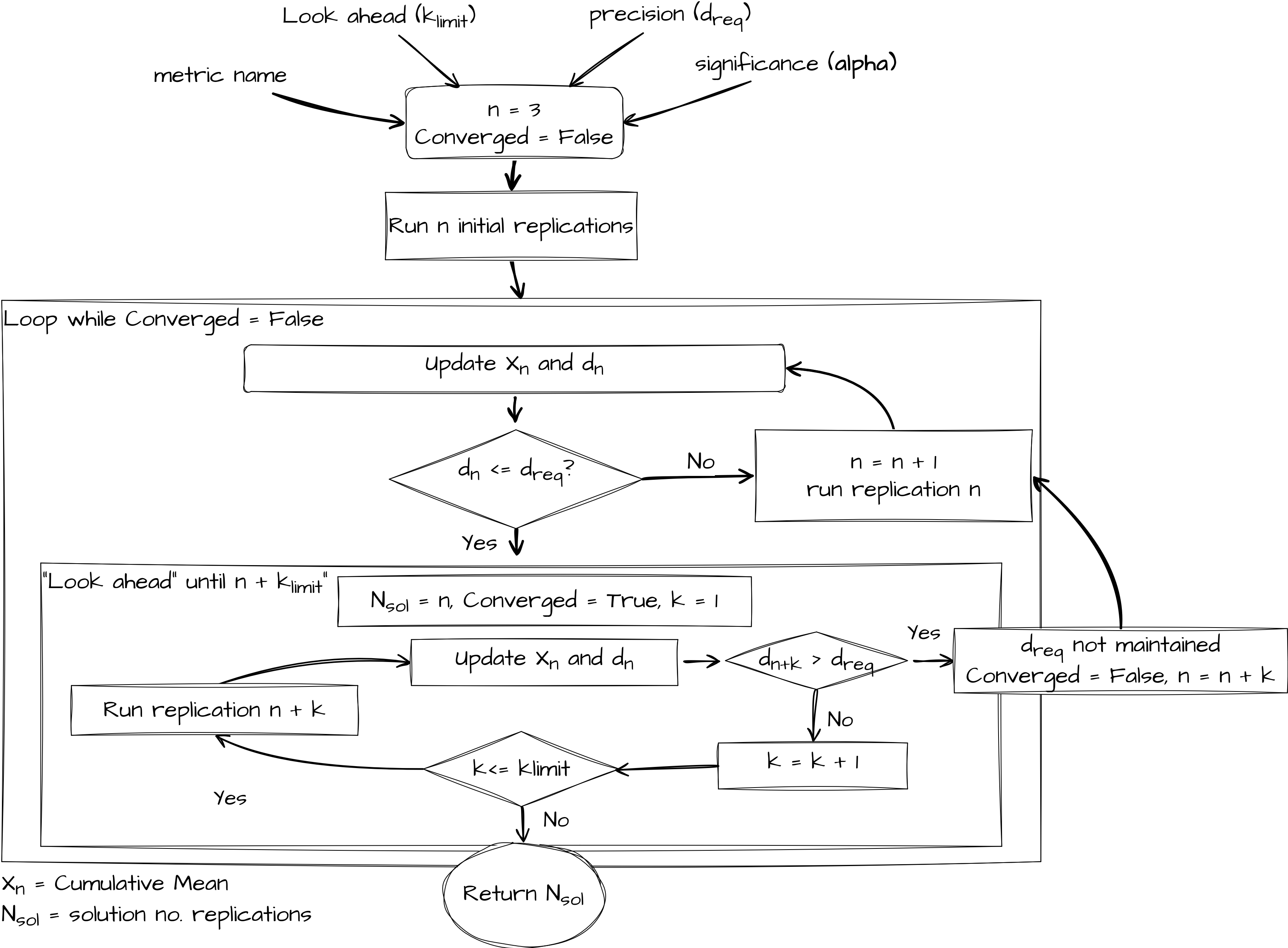
The sim-tools package includes an implementation of the “replications algorithm” from Hoad, Robinson, & Davies (2010), used to automatically determine the number of simulation replications needed to achieve a user-specified confidence interval (CI) precision. It works by combining:
- The confidence interval method (described on the previous page), which estimates the required replications for a target CI half-width.
- A sequential look-ahead procedure to check whether the desired CI precision is still met as additional replications are run.
If you make use of this code in your work please cite the sim-tools as well as the original authors article:
Hoad, Robinson, & Davies (2010). Automated selection of the number of replications for a discrete-event simulation. Journal of the Operational Research Society. https://www.jstor.org/stable/40926090
Note: The examples below use the treat-sim model. If you haven’t run it before, see Using the example treat-sim model for set-up and basic usage.
Imports
Replications Algorithm overview
The look ahead component is governed by the formula below. A user specifies a look ahead period called \(k_{limit}\). If \(n \leq 100\) then a parameter \(k_{limit}\) is used. Hoad et al.(2010) recommend a value of 5 based on extensive empirical work. If \(n \geq 100\) then a fraction is returned. The notation \(\lfloor\) and \(\rfloor\) mean that the function must return an integer value (as it represents the number of replications to look ahead).
\[ f(k_{limit}, n) = \left\lfloor \dfrac{k_{limit}}{100}\max(n, 100)\right\rfloor \]
In general \(f(k_{limit}, n)\) means that as the number of replications increases so does the look ahead period. For example when you have run 50 replications a \(k_{limit} = 5\) means you simulate an extra 5 replications. When you have run 800 replications, a \(k_{limit} = 5\) means the number of extra replications you simulate is:
\[ \left\lfloor \dfrac{5}{100} \times 800\right\rfloor = 40 \]
The paper provides a formal algorithm notation. Here we provide a pictorial representation of the general logic of the replications algorithm.
Observers
The ReplicationAlgorithm requires an observer. This is an object whose job it is to watch each replication in your algorithm and record relevant statistics as the simulation runs.
A suitable observer is supplied by default - ReplicationTabulizer - but you can also create your own, but it needs to follow this protocol:
@runtime_checkable
class AlgorithmObserver(Protocol):
    """
    Protocol for observer classes used in ReplicationsAlgorithm.

    Classes implementing this protocol should provide a `dev` attribute
    to store observations, a method `update` to add new results, and a
    `summary_table` method to summarize the stored replication statistics.

    Attributes
    ----------
    dev : List[Any]
        Collection of observed replication results.

    Methods
    -------
    update(results) -> None
        Add an observation of a replication.

    summary_table() -> pd.DataFrame
        Create a DataFrame summarising all recorded replication statistics.
    """

    dev: List[Any]

    def update(self, results) -> None:
        ...

    def summary_table(self) -> pd.DataFrame:
        ...
What does this mean?
AlgorithmObserver essentially just tells us that:
- There should be a
.devattribute containing the percentage deviation. - There should be an update() method which updates statistics after each replication.
- There should be a summary_table() method which returns a dataframe summarising the replication results.
Adapting a simulation model to work with ReplicationsAlgorithm
Why an adapter is needed
Every simulation model has it’s own way of:
- Being initialised (parameters, scenario set-up)
- Running a single replication (function/method name, arguments)
- Returning results (scalar, dict,
DataFrame, etc.)
The ReplicationsAlgorithm needs to be able to call any model in a consistent way, regardless of those differences. To do that, we need to wrap models in an Adapter - a “wrapper” object exposing a fixed interface the algorithm can use.
Required interface
We formalise what the adapter must look like with a Protocol called ReplicationsAlgorithmModelAdapter.
@runtime_checkable
class ReplicationsAlgorithmModelAdapter(Protocol):
    """
    Adapter pattern for the "Replications Algorithm".

    All models that use ReplicationsAlgorithm must provide a
    single_run(replication_number) interface.
    """

    def single_run(self, replication_number: int) -> dict[str, float]:
        """
        Run a single unique replication of the model and return results.

        Parameters
        ----------
        replication_number : int
            The replication sequence number.

        Returns
        -------
        dict[str, float]
            {'metric_name': value, ... } for all metrics being tracked.
        """
        pass
What does this mean?
ReplicationsAlgorithmModelAdapter essentially just tells us that:
- There should be a single_run() method which is passed the
replication_numberto seed it. - It should return a dictionary mapping metric name to float value for every requested metric, after just one replication.
Adapter for treat-sim
Below is an adapter for the treat-sim model.
# pylint: disable=too-few-public-methods
class TreatSimAdapter:
    """
    treat-sim multi-metric single_run interface adapter for the
    ReplicationsAlgorithm.
    """

    def __init__(
        self,
        scenario: Scenario,
        metrics: list[str],
        single_run_func: Callable,
        run_length: Optional[float] = 1140.0,
    ):
        """
        Parameters:
        ------------
        scenario: Scenario
            The experiment and parameter class for treat-sim

        metrics: list[str]
            The metric(s) to output

        single_run_func: Callable
            The single run function that is being adapted.
            This must return something indexable by metric name.

        run_length: float, optional (default = 1140)
            The run_length for the model
        """
        self.scenario = scenario
        self.metrics = metrics
        self.single_run_func = single_run_func
        self.run_length = run_length

    def single_run(self, replication_number: int) -> dict[str, float]:
        """
        Conduct single run of the simulation.
        Returns a dictionary of {metric_name: value}.
        """
        results_df = self.single_run_func(
            self.scenario,
            rc_period=self.run_length,
            random_no_set=replication_number,
        )
        return {metric: results_df[metric].iloc[0] for metric in self.metrics}
Note that TreatSimAdapter does what is says on the tin: it adapts the model so that its implements the expected interface. I.e.
METRICS = ["01a_triage_wait", "01b_triage_util", "02a_registration_wait"]

ts_model = TreatSimAdapter(
    scenario=Scenario(), metrics=METRICS, single_run_func=single_run
)

ts_model.single_run(1)
{'01a_triage_wait': np.float64(57.120114285877285),
'01b_triage_util': np.float64(0.6213484543463906),
'02a_registration_wait': np.float64(90.00238510732363)}The Protocol ReplicationsAlgorithmModelAdapter is marked as @runtime_checkable, which allows us to check at runtime that any supplied model conforms to the expected interface.
print(isinstance(ts_model, ReplicationsAlgorithmModelAdapter))TrueExample usage
Running ReplicationsAlgorithm on a single metric
# Set up model with adapter
ts_model = TreatSimAdapter(
    scenario=Scenario(), metrics=["01a_triage_wait"], single_run_func=single_run
)

# Run algorithm
analyser = ReplicationsAlgorithm(observer_factory=ReplicationTabulizer)
nreps, summary_frame = analyser.select(model=ts_model, metrics=["01a_triage_wait"])

# Preview results
print(nreps)
summary_frame.head()
{'01a_triage_wait': 145}| Mean | Cumulative Mean | Standard Deviation | Lower Interval | Upper Interval | % deviation | metric | |
|---|---|---|---|---|---|---|---|
| 0 | 24.280943 | 24.280943 | NaN | NaN | NaN | NaN | 01a_triage_wait |
| 1 | 57.120114 | 40.700529 | NaN | NaN | NaN | NaN | 01a_triage_wait |
| 2 | 28.659383 | 36.686814 | 17.830662 | -7.607007 | 80.980634 | 1.207350 | 01a_triage_wait |
| 3 | 24.801392 | 33.715458 | 15.724847 | 8.693717 | 58.737199 | 0.742144 | 01a_triage_wait |
| 4 | 17.679156 | 30.508198 | 15.391092 | 11.397633 | 49.618763 | 0.626408 | 01a_triage_wait |
You can visualise the tabulized results using the plotly_confidence_interval_method function.
plotly_confidence_interval_method(
    n_reps=nreps["01a_triage_wait"],
    conf_ints=summary_frame[summary_frame["metric"] == "01a_triage_wait"],
    metric_name="01a_triage_wait",
)
Running ReplicationsAlgorithm on a multiple metrics
METRICS = ["01a_triage_wait", "01b_triage_util", "02a_registration_wait"]

# Set up model with adapter
ts_model = TreatSimAdapter(
    scenario=Scenario(), metrics=METRICS, single_run_func=single_run
)

# Run algorithm
analyser = ReplicationsAlgorithm(observer_factory=ReplicationTabulizer)
nreps_m, summary_frame_m = analyser.select(model=ts_model, metrics=METRICS)

# Preview results
print(nreps_m)
summary_frame_m.head()
{'01a_triage_wait': 145, '01b_triage_util': 4, '02a_registration_wait': 16}| Mean | Cumulative Mean | Standard Deviation | Lower Interval | Upper Interval | % deviation | metric | |
|---|---|---|---|---|---|---|---|
| 0 | 24.280943 | 24.280943 | NaN | NaN | NaN | NaN | 01a_triage_wait |
| 1 | 57.120114 | 40.700529 | NaN | NaN | NaN | NaN | 01a_triage_wait |
| 2 | 28.659383 | 36.686814 | 17.830662 | -7.607007 | 80.980634 | 1.207350 | 01a_triage_wait |
| 3 | 24.801392 | 33.715458 | 15.724847 | 8.693717 | 58.737199 | 0.742144 | 01a_triage_wait |
| 4 | 17.679156 | 30.508198 | 15.391092 | 11.397633 | 49.618763 | 0.626408 | 01a_triage_wait |
for metric in METRICS:
    mask = summary_frame_m["metric"] == metric
    fig = plotly_confidence_interval_method(
        n_reps=nreps_m[metric],
        conf_ints=summary_frame_m[mask].reset_index(),
        metric_name=metric,
    )
    fig.show()